2. Aerospace Projects
Key Skills
Mission Design, Orbital Mechanics, Systems Engineering, Propulsion Analysis, High-Power Rocketry (Design, Build, Fly)
Core Tools
MATLAB, Python, SolidWorks, OpenRocket, Composite Fabrication
Hands-on aerospace experience is essential for bridging theoretical knowledge with practical engineering challenges. This section highlights my involvement in high-power rocketry and professional aerospace systems engineering through an internship at Lockheed Martin.
2.1 High Power Rocketry: "Wave Function"
As Secretary of the Mines Rocket Club, I apply engineering principles to personal projects. The "Wave Function" rocket was my Level 2 high-power certification flight, encompassing the full design, fabrication, and flight operations cycle.
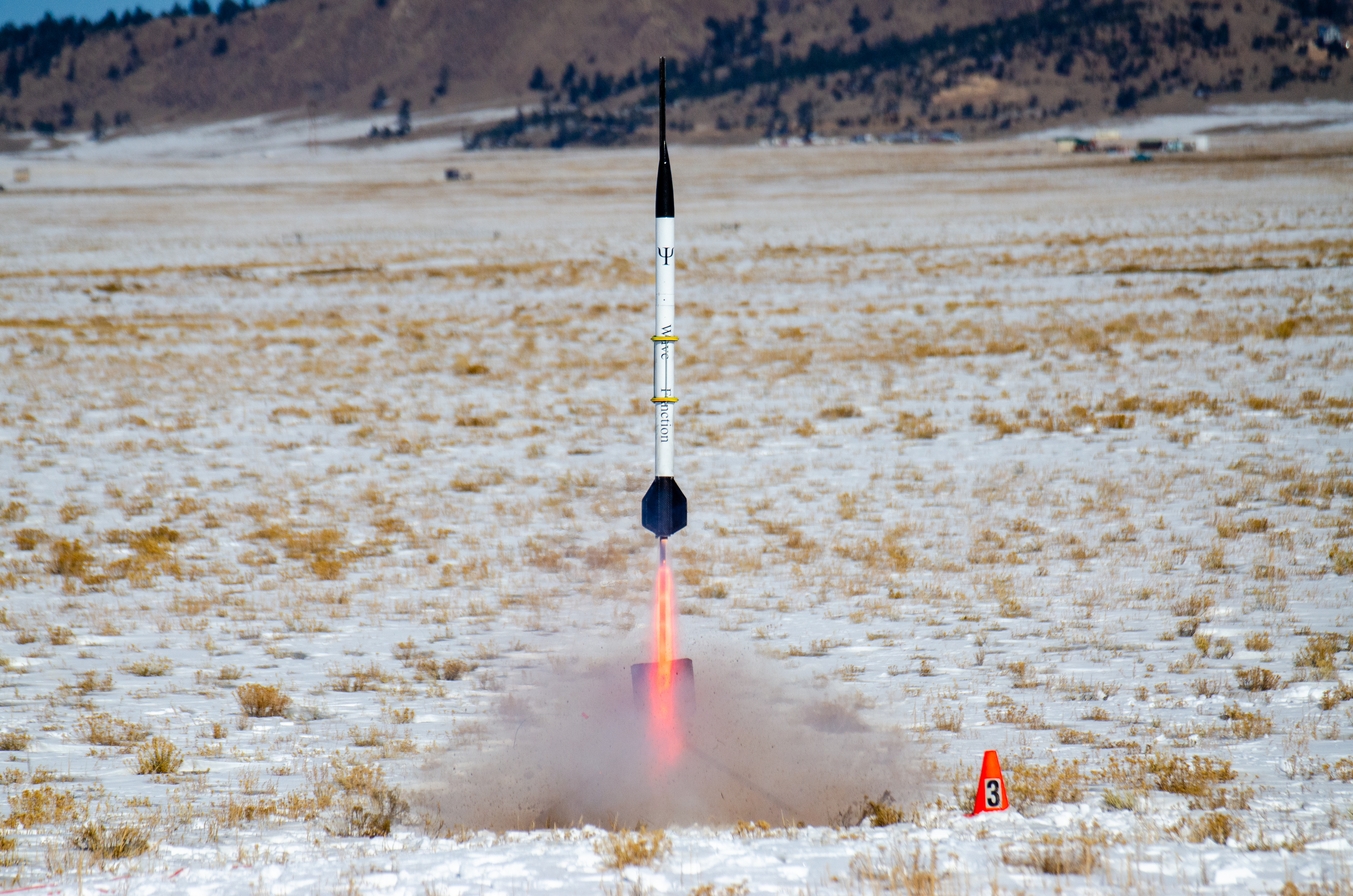
Rocket Specifications
- Overall length: 1.4 meters
- Body diameter: 98 mm (4 inches)
- Loaded Mass: 5.2 kg
- Motor: Cesaroni Pro75 L1115
- Stability: 2.1 calibers
Flight Performance
- Launch Date: Nov 17, 2025
- Peak Altitude: 12,794 ft AGL
- Max Velocity: 2,312 ft/s
- Recovery: Dual-deployment (drogue at apogee, main at 900 ft).
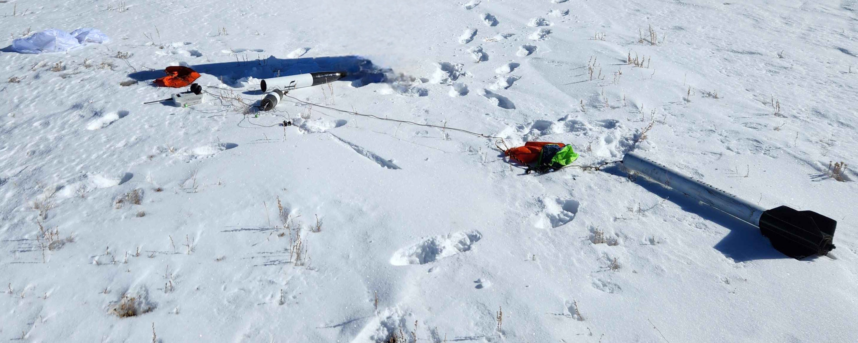
2.1.2 Custom Components
- Nose Cone: 3D-printed, two-piece Haack series cone (detailed in Chapter 1) designed to fit printer build volume.
- Fins: Four 1/4-inch G10 fiberglass fins with through-the-wall construction and internal fillets for structural integrity.
- Recovery System: Dual-deployment using CO₂ ejection, a Tender Descender device, and a 36-inch main parachute.
- Avionics: Featherweight Raven4 altimeter for flight data acquisition and deployment control.
Post-Flight Analysis: The flight demonstrated excellent stability. Comparison between OpenRocket predictions and altimeter data revealed a **95% accuracy in altitude prediction**. This project provided invaluable hands-on experience with the complete engineering design cycle.
2.2 Lockheed Martin Space Internship
During my internship, I served as the Payload & Mission Design Lead on a five-person intern team. I pitched the concept for the "Mercury Ice Flayer" mission, a smallsat orbiter designed to investigate ice deposits at Mercury's north pole.
My responsibilities included designing the primary payload (the "NIMI" infrared spectrometer), defining the scientific rationale, performing a propulsion trade study, and researching launch vehicles. The most challenging part was teaching myself MATLAB to develop the orbital trajectory and launch window analysis required to prove the mission's feasibility.
Final Presentation
Our team won the intern design competition with our final presentation, which details the full mission architecture.
View Presentation (.pdf)
Propulsion Trade Study
I conducted this trade study comparing five propulsion systems for our 190kg smallsat's capture at Mercury.
View Trade Study (.pdf)
Mercury Launch Window Analysis
A critical component of my mission design work was this comprehensive trajectory analysis to find feasible Earth-to-Mercury launch windows. The full study was written in LaTeX, and the analysis was performed with a custom, toolbox-free MATLAB suite I developed.
Key Results
Identified optimal 2028-2029 launch windows with C3 < 60 km²/s² and Mercury arrival velocities v∞ < 10 km/s, suitable for small-satellite rideshare missions.
Analysis Methodology
Baseline Transfer: Hohmann Analysis
A Hohmann transfer provides first-order feasibility bounds. For circular coplanar orbits at r1 = 1.000 AU (Earth) and r2 = 0.387 AU (Mercury):
This establishes expectations: transfer time ≈ 105 days, C3 ≈ 15 km²/s², and Mercury arrival Δv ≈ 7 km/s.
Lambert Problem Implementation
Algorithm
The core trajectory computation solves Lambert's problem using the universal variable formulation. Given position vectors r1, r2 and time of flight Δt, the solver determines velocity vectors v1, v2 by iterating on the universal anomaly z:
where C(z) and S(z) are Stumpff functions.
Downloadable Source Code
The full MATLAB suite used for this analysis is available for download. All code is toolbox-free and relies on the function-based architecture detailed below.
Code Showcase: lambert_universal.m
The core of the analysis is this single-revolution, toolbox-free Lambert solver based on the universal variable formulation.
function [v1, v2, ok] = lambert_universal(r1, r2, dt, mu, prograde)
% LAMBERT_UNIVERSAL  Single-revolution Lambert solver (toolbox-free).
% r1,r2 [m], dt [s], mu [m^3/s^2], prograde true/false
% Returns v1,v2 [m/s], ok boolean.

ok   = false;
v1   = nan(3,1);
v2   = nan(3,1);

r1n = norm(r1);
r2n = norm(r2);
if dt <= 0 || r1n == 0 || r2n == 0, return; end

% Transfer angle
cos_dnu = dot(r1, r2) / (r1n * r2n);
cos_dnu = max(-1, min(1, cos_dnu));
sin_dnu = norm(cross(r1, r2)) / (r1n * r2n);
if ~prograde, sin_dnu = -sin_dnu; end
dnu = atan2(sin_dnu, cos_dnu);
if dnu <= 0, dnu = dnu + 2*pi; end   % enforce positive transfer angle

% Battin/Prussing-Conway form
A = sin(dnu) * sqrt(r1n * r2n / (1 - cos_dnu));
if abs(A) < eps, return; end

% Solve for z with Newton on
% F(z) = ( (y/C)^1.5 )*S + A*sqrt(y) - sqrt(mu)*dt = 0
z    = 0.0;             % reasonable start
tol  = 1e-8;
itmx = 100;

for it = 1:itmx
  [Cz, Sz] = stumpff(z);
  % y(z)
  if Cz <= 0, z = z + 0.1; continue; end
  y = r1n + r2n + A * (z*Sz - 1) / sqrt(Cz);
  if y <= 0
    % push z toward positive where y tends to grow
    z = z + 0.1;
    continue
  end

  % F(z)
  chi = sqrt(y / Cz);
  F   = chi^3 * Sz + A * sqrt(y) - sqrt(mu) * dt;
  if abs(F) < tol
    break
  end

  % ... (Derivative calculation and Newton step) ...

end

% ... (Final y check and Lagrange coefficient calculation) ...

f    = 1 - y / r1n;
g    = A * sqrt(y / mu);
gdot = 1 - y / r2n;

if abs(g) < 1e-9 || ~isfinite(g), return; end

v1 = (r2 - f * r1) / g;
v2 = (gdot * r2 - r1) / g;
ok = all(isfinite([v1; v2]));
end

function [C, S] = stumpff(z)
% STUMPFF  Safe Stumpff functions C(z), S(z)
if z > 1e-3
  s = sqrt(z);
  S = (s - sin(s)) / (s^3);
  C = (1 - cos(s)) / z;
elseif z < -1e-3
  s = sqrt(-z);
  S = (sinh(s) - s) / (s^3);
  C = (cosh(s) - 1) / (-z);
else
  % series for small |z|
  z2 = z*z;
  C  = 1/2 - z/24 + z2/720 - z*z2/40320;
  S  = 1/6 - z/120 + z2/5040 - z*z2/362880;
end
end
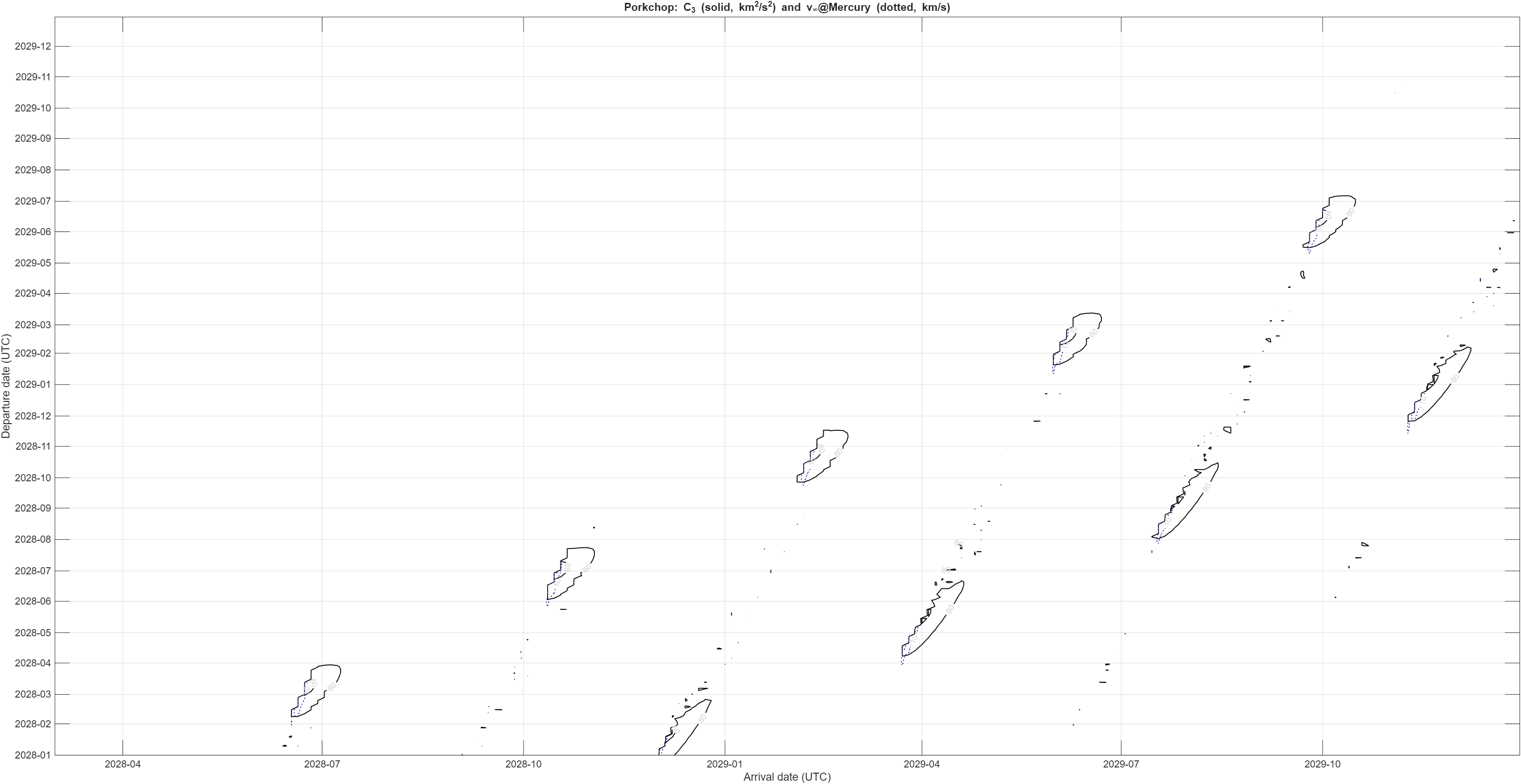
Launch Window Optimization
Porkchop Plot Generation
The analysis grids departure and arrival dates, solving Lambert's problem at each point to compute:
Mercury Orbit Insertion
The chemical propulsion Δv required to capture into an elliptical Mercury orbit is:
For our 80 km x 2000 km polar orbit with v∞ = 9.6 km/s, Δvcap ≈ 2.3 km/s.
Optimal Transfer Windows
Top Candidates (2028-2029)
| Departure | Arrival | ToF [d] | C3 [km²/s²] | v∞,M [km/s] |
|---|---|---|---|---|
| 2028-10-27 | 2029-02-09 | 105 | 56.83 | 9.63 |
| 2029-06-12 | 2029-09-28 | 108 | 57.05 | 9.62 |
| 2028-06-29 | 2028-10-15 | 108 | 57.15 | 9.63 |
The best window (Oct 27, 2028 → Feb 9, 2029) offers C3 = 56.8 km²/s², compatible with ESPA-class rideshare opportunities, and v∞ = 9.6 km/s, enabling capture with modest propulsion systems.